|
So those look pretty cool, or so I like to think. But how did I do it? You'll be interested to know that it was all coordinate geometry, really. Basically I spent a whole day thinking back to my high school classes, working out how to produce the frames that I would put together to create animated spins of the structures that I had found. And then another day writing it all in code. But the code isn't the story here, we'll focus on the mathematics involved. To create an animation of anythng, we first need to produce still frames, and in this case I needed each frame to show the structure from a specific angle. For each of these frames, we need to project the three-dimensional positions of the parts of each structure onto a viewing plane. Then we need to rotate the structure (or equivalently, revolve our camera) by some regular angular increment, and for a nice touch to enforce the three-dimensional feel of the animation, put it all in a box. You would have already seen the completed animations that I linked to above, but here's a basic "skeletal" example, of the solid-particle-render variety. 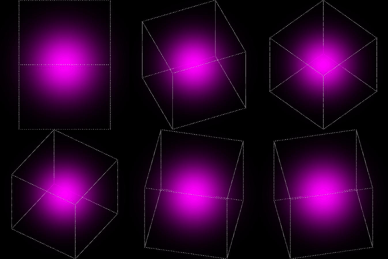 Two things to note in particular are that:
Here's another skeletal example: 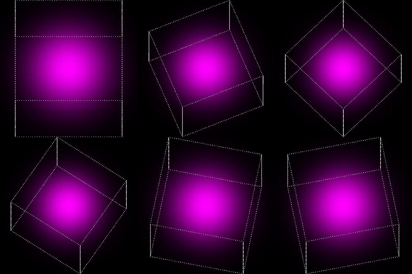 What we've changed here is that the angle of elevation of the camera's revolution is closer to one of the "poles". To achieve this, we need to put the camera at the correct "height", and there is a relation between angle and gradient that we need here. So what we have seen is that in three-dimensional modelling, coordinate geometry is essential. I myself used it to to create lines (intervals), distinguish background and foreground objects and relate angles to horizontal and vertical displacements. Below I reprise some finished products - both show the scale of homogeneity, a scale at which the Universe is thought to be homogeneous. A solid particle render: 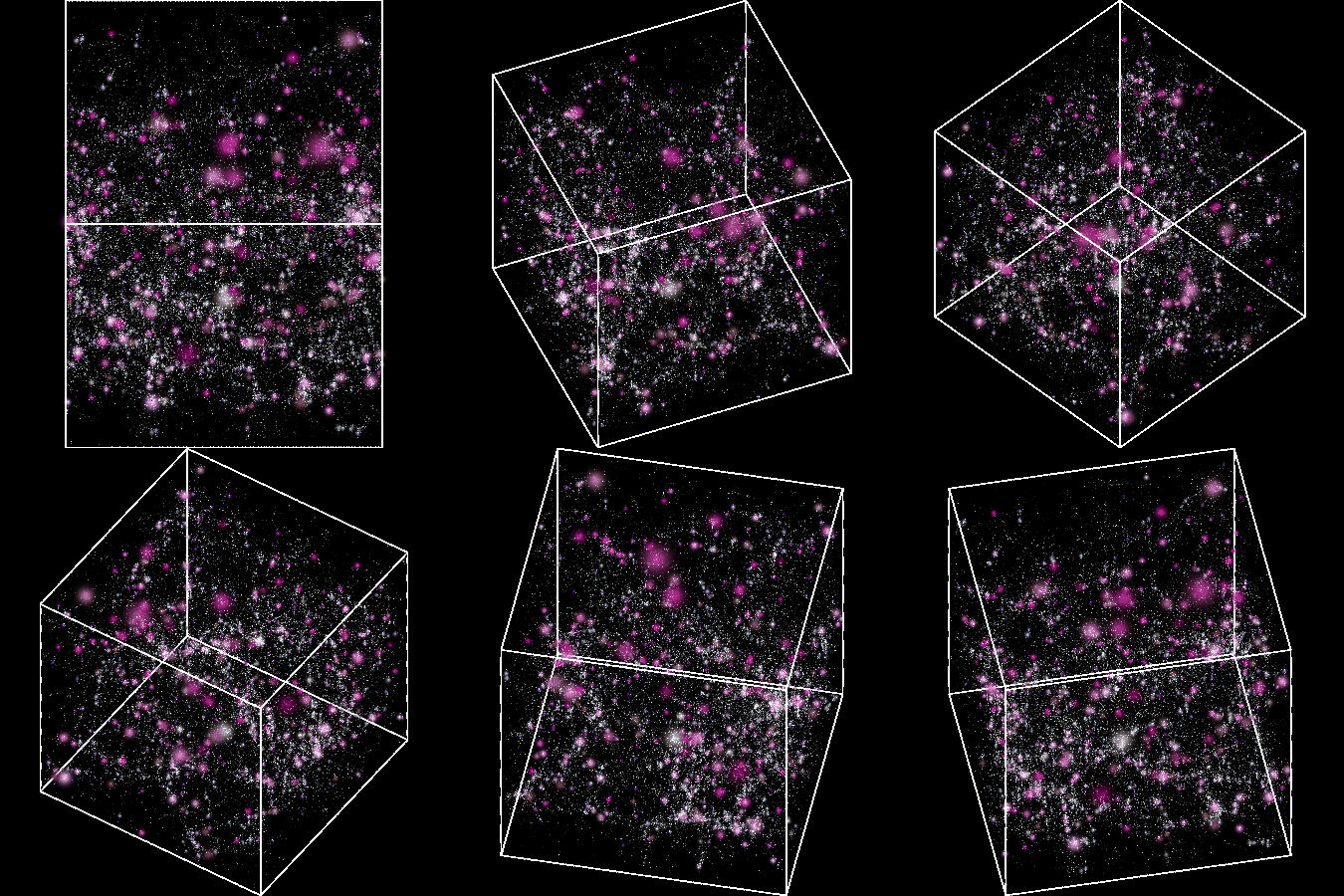 An isosurface, which is a different mode of visualisation to what we have looked at above, but the same principles still apply: 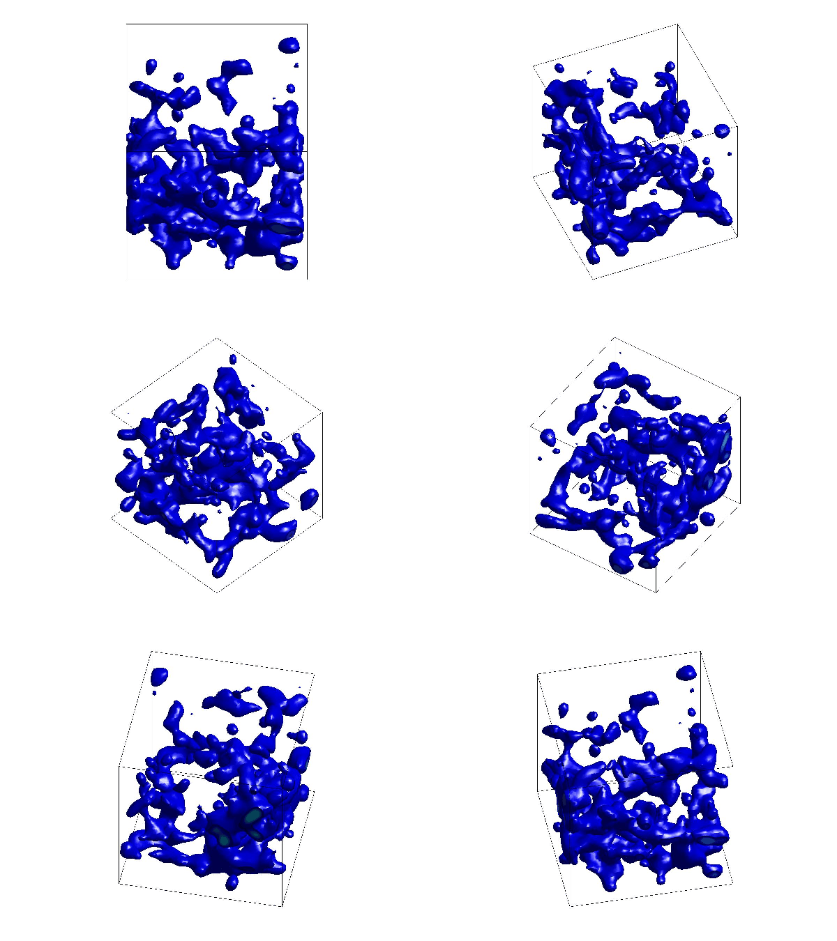 |